Figures from Willett et al. 2013


| Met Office Hadley Centre observations datasets |
| > Home > HadISDH > |
Please read the paper before using the material presented here.
All figures have been created using HadISDH.landq.1.0.0.2012p and are under Crown Copyright. Please acknowledge use of this material using the following reference:
Willett, K. M., Williams Jr., C. N., Dunn, R. J. H., Thorne, P. W., Bell, S., de Podesta, M., Jones, P. D., and
Parker D. E., 2013: HadISDH: An updated land surface specific humidity product for climate monitoring.
Climate of the Past, 9, 657-677, doi:10.5194/cp-9-657-2013. PDF file (5.4MB)
| Title | Description | Link | Images |
|---|---|---|---|
|
Figures from Willett et al. 2013
|
|||
| Fig. 1 HadISDH Station Coverage | Station coverage comparison between HadCRUH and HadISDH. a) Station coverage in HadISDH. Stations in red/pink were also in HadCRUH. Stations in blue/turquoise are new. Pink and turquoise stations are stations that are composites of more than one original source station. b) Stations from HadCRUH that are no longer in HadISDH (dark green) and HadISDH stations with subzero specific humidity issues after homogenisation that are not included in any further analyses (light green). c) Station coverage by month for HadISDH, coloured by region (N. Hemisphere = 20°N-90°N, Tropics = 20°S-20°N, S. Hemisphere = 20°S-90°S). The tail-off from 2006 onwards is likely due to ongoing improvements to the ISD historical archive. Station coverage should improve over this period with future updates of HadISDH. | Fig1_HadISDHPHA_coverageFEB2013.png | |
| Fig. 2 Quality control data removal | Percentage of hourly observations removed for each HadISDH station during the HadISD quality control procedure for a) temperature and b) dewpoint temperature. | Fig2a_ALL_T_mapfails_hadcruh_20130215.png Fig2b_ALL_Td_mapfails_hadcruh_20130215.png | |
| Fig. 3 Homogeneity adjustments - time, magnitude | Summary of adjustments applied to HadISDH during the pairwise homogenisation process. Figure a) shows the actual adjustments in black (stepped). The best-fit Gaussian is shown in grey. The merged Gaussian plus larger actual distribution points 'best-fit' is shown in dashed red. The difference between the merged 'best-fit' and the actual adjustments is shown in dotted blue with the mean and standard deviation of the difference. | Fig3_HadISDH_adjspread_FEB2013.png | |
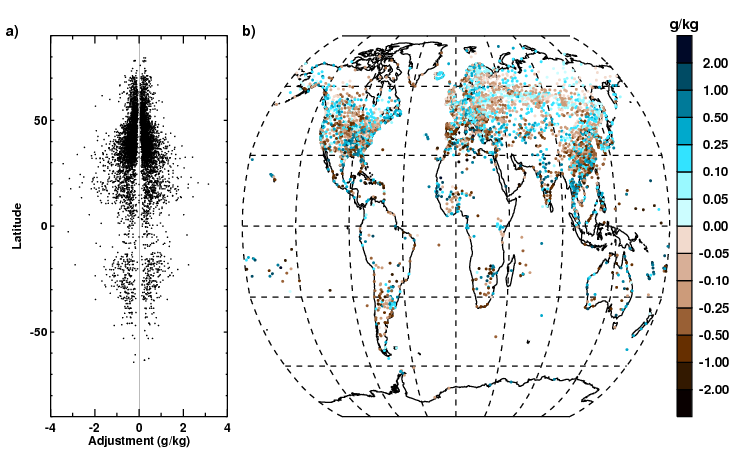
| Fig. 4 Homogeneity adjustments - location, magnitude | Distribution of adjustments made and their magnitude during the pairwise homogenisation process: a) adjustments by latitude; b) largest adjustments for each station. Note non-linear colour bars. | Fig4_HadISDH_adjspreadmaps_FEB2013.png | |
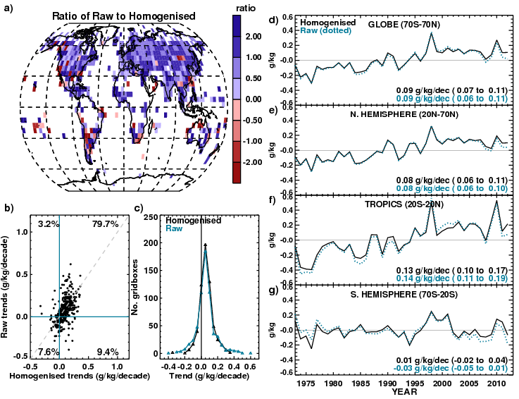
| Fig. 5 Homogeneity adjustments - raw vs. adjusted | Difference between trends (1973-2012) in HadISDH before and after the pairwise homogenisation process. a) Ratio of decadal trends from the raw HadISDH compared to homogenised HadISDH (trend methodology is described in Figure 9). Note non-linear colour bars. b) Scatter relationship between homogenised and raw decadal trends for HadISDH. The percentage of gridboxes present in each quadrant is shown. c) Distribution of grid-box trends for the homogenised and raw data. d-g) Large-scale area average annual anomaly time series and trends for homogenised HadISDH and the raw data relative to the 1976-2005 climatology period. | Fig5_HadISDHPHAFLAT_MPtrendsscat_FEB2013.png | |
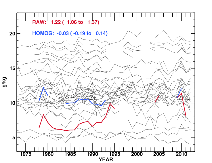
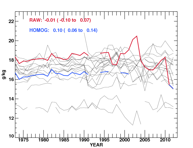
| Fig. 6 Homogeneity adjustments - example stations | Results for three stations as examples of some of the largest changes of the pairwise homogenisation algorithm. Red lines represent the original station time series. Blue lines represent the adjusted time series. Black lines show the original time series for all stations within the designated network. a) Sur, Oman, WMO ID: 412680, 22.533°N, 59.467°E, 14.0m. b) Atar, Mauritania, WMO ID: 614210, 20.5170°N, 13.0670°W, 224.0m. c) Sao Luiz, Brazil, WMO ID: 822810, 2.6000°S, 44.2330°W, 53.0m. | Fig6a_41268099999_trendcomp_7312Feb2013.png Fig6b_61421099999_trendcomp_7312Feb2013.png Fig6c_82281099999_trendcomp_7312Feb2013.png | |
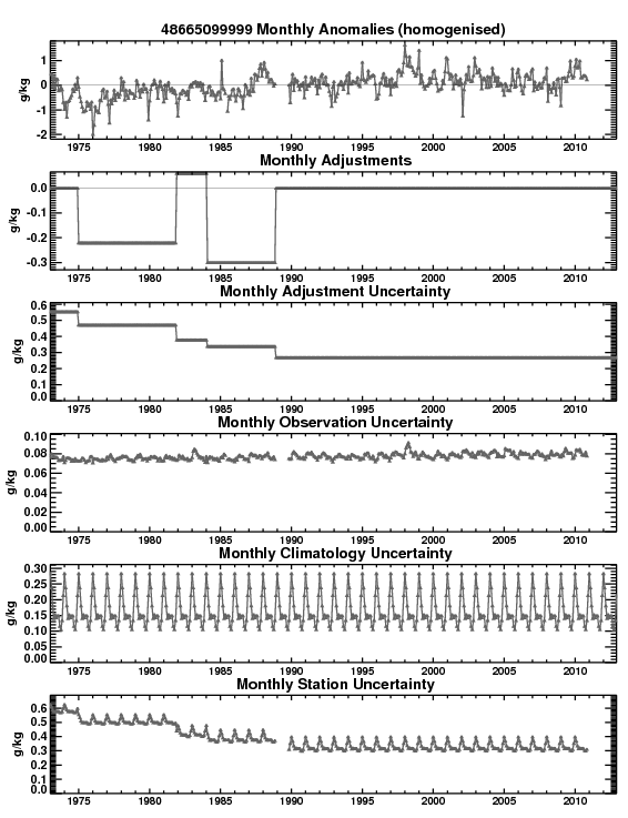
| Fig. 7 Station uncertainty - example station | The components of station uncertainty estimates for station 486650 (Malacca, Malaysia, 2.267°N, 102.250°E, 9.0m). All uncertainties represent 2? (approximately 95 % confidence intervals). | Fig7_48665099999_stationstatsFEB2013.png | |
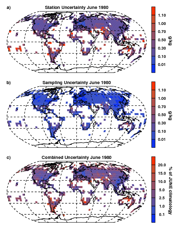
| Fig. 8 Gridbox uncertainty | Gridded 2 sigma uncertainty fields for HadISDH. a) June 1980 gridded station uncertainty, b) sampling uncertainty, c) combined uncertainty for June 1980 as a percentage of the grid-box climatological (1976-2005) value for June. Note non-linear colour bars. | Fig8_HadISDHPHAFLAT_uncertainty_FEB2013.png | |
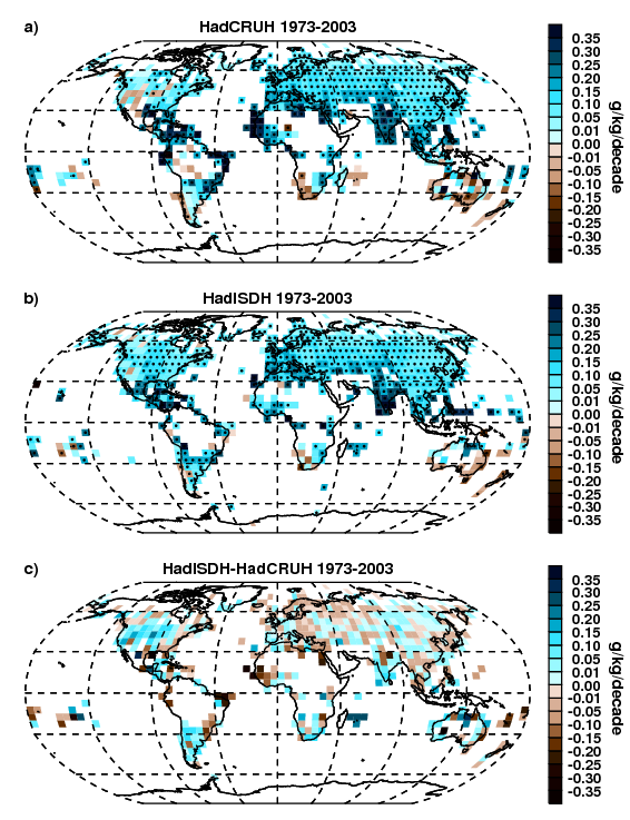
| Fig. 9 Gridbox decadal trends - compared to HadCRUH 1973-2003 | Decadal trends in specific humidity for HadCRUH verses HadISDH over the 1973-2003 period of record. Trends have been estimated using the median of pairwise slopes (Sen 1968; Lanzante 1996) method. Where intervals defined by the 95 % confidence limits on the median of the slopes are both of the same sign as the median trend presented in the gridboxes the trend is presumed to be significantly different from a zero trend. This is indicated by a black dot within the gridbox. This means that there is higher confidence in the direction of the trend, but not necessarily the magnitude. The spread of the confidence interval provides the confidence in the magnitude, these values are available online at www.metoffice.gov.uk/hadobs/hadisdh. Note non-linear colour bars. | Fig9_HadISDHPHAFLAT_MPdectrendsCOMP_FEB2013.png | |
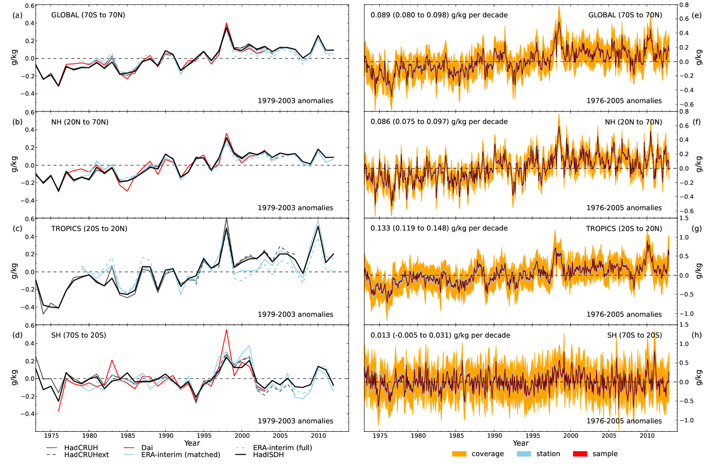
| Fig. 10 Monthly and annual time series and decadal trends | Time series of large-scale average specific humidity over land for HadISDH and existing data-products. a-d) Annual time series from all other global surface humidity products given a zero mean over the common period of 1979-2003. Dai covers 60°S to 70°N. ERA-Interim has been weighted by % land coverage in each gridbox and is shown both spatially matched to HadISDH and with complete coverage. e-h) Monthly time series (relative to the 1976-2005 climatology period) for HadISDH with 2 sigma uncertainty estimates. The black line is the area average (using weightings from the cosine of the latitude). The red, blue and orange lines show the +/- combined uncertainty estimates from the grid-box sampling uncertainty, the station uncertainty and the spatial coverage uncertainty respectively. Trends are shown for each region for the period 1973-2012. These have been fitted using the median of pairwise slopes as described in Figure 9 with the 95 % confidence intervals shown. Where these are both of the same sign (i.e., the globe, Northern Hemisphere and tropics) there is high confidence that trends are significantly different from zero. | .Fig10_hadcruh_uncertainties.pngpng | |
| Fig. 11 Gridbox decadal trends 1973-2012 | Decadal trends in specific humidity for HadISDH over 1973-2012. Trends are fitted and confidence assigned as described in Figure 9. Note non-linear colour bars. | Fig11_HadISDHPHAFLAT_MPdectrends_FEB2013.png.png | |
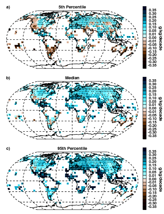
| Fig. 12 Exploring uncertainty in gridbox decadal trends | Exploration of the uncertainty in decadal trends using 100 realisations of HadISDH spread across the 2 sigma uncertainty estimates. Median pairwise trends were fitted over the period for each realisation, with higher confidence assigned by a black dot as described in Figure 9. For each gridbox, the 5th percentile (a), median (b) and 95th percentile (c) trends are shown. If the uncertainty was large enough to obscure the long-term trends then it would be expected that the 5th and 95th percentiles would starkly disagree with each other. In fact, there is very little difference as shown by a, b and c above. Note non-linear colour-bars. | Fig12_HadISDHPHAFLAT_MPdectrendsUNC_FEB2013.png.png | |
| Fig. 13 Annual average time series and uncertainties compared with temperature | Comparison of large scale annual average time series from HadISDH land specific humidity with land surface air temperature from CRUTEM4 (Jones et al. 2012) and sea surface temperature from HadSST3 (Kennedy et al. 2011a, b) including uncertainty ranges. Temperature data have been adjusted to have a zero-mean over the 1976-2005 climatology period of HadISDH. Correlations between the land air temperature and SST and land surface humidity have been performed on the detrended time series. | Fig13_HadISDH_tempsTS_FEB2013.png | |
| Fig. 14 Moist years vs warm years | Annual average anomalies (from the 1976-2005 climatology period) for HadISDH specific humidity and HadCRUT4 (Morice et al. 2012) temperature, for the two moistest years within the HadISDH record (1998 and 2010) which were also among the warmest years since records began in 1850, and one of the warmest years in the land record from CRUTEM4 (2007: see Figure 13) that was not simultaneously very moist. Note non-linear colour bars. | Fig14_HadISDHPHAFLAT_moistyears_FEB20133maps.png | |
Further plots and text will appear here over time
 |
Maintained by: Kate Willett |
© Crown Copyright
|